More blue water - why is the Nil Diya Pokuna blue?

On my last visit to Sri Lanka, I was keen on exploring some lesser-known attractions and decided to visit Nil Diya Pokuna (නිල් දිය පොකුණ) located close to Ella in the Uva Province. I was impressed and fascinated by the massive underground cave complex and the blue water pond at the end of the 850m hike through the cave. This was the second time I saw clear blue water in Sri Lanka, the first being in a limestone quarry.  

The usual reason for ponded water to appear bright blue or turquoise in colour is the fine particulates that selectively scatter light through water (the same reason why the sky is blue). In the case of the limestone quarry the fine particulates are minute calcite crystals and in the case of glacial lakes they are finely ground rock particles known as glacial flour. 

Nil Diya Pokuna has a very interesting geology, with several different rock types present around and within the caves, and I wanted to understand what gives the water its blue colour. Caves of this scale are usually formed by the action of weathering and erosion of sedimentary rocks such as limestone. However, this region of Sri Lanka consists of primary of metamorphic rocks. This blog post by Dr Jayasingha describes the geological origins of the cave complex containing Nil Diya Pokuna. According to it, the caves have been formed by the initial dissolution of Marble, which leads to weakening of rock joints and bedding planes and subsequent collapses of the other rock masses creating the large underground caverns. 

Marble is formed by the metamorphosis of limestone, and its dissolution would lead to the release of calcite crystals. There are stalactites formed at several places within the cave, as seen in the photos below, that confirm the occurrence of marble or limestone dissolution. Therefore, it is reasonable to conclude that the reason for the blue coloured water in Nil Diya Pokuna is the calcite crystals that are accumulated in the water as it flows through the joints and fissures in rock containing marble or limestone before making its way into the pond. Below are some photos from my visit:

Stalactites in the cave indicating marble or limestone dissolution
 

Evidence of weathering and staining in the rock

Visible bedding planes and smooth joint surface of a possible collapse leading to cave formation

Blue water and more stalactites

High water levels were blocking off some more expansive areas of the cave

The water was a little murky due to recent rains

Estimating surface settlement induced by underbore or tunnel construction

It is often necessary to estimate the potential ground surface settlement caused by underground infrastructure projects involving tunnels and underbores. Such settlement assessments are used to determine if any additional protection works are necessary particularly if underbores are tunnels are to be constructed underneath roads, railways or buildings. Finite element analysis programs such as Plaxis 2D/3D, Optum G2/G3 or FLAC are typically used to model settlements in such instances. Accurate information on ground properties, tunnel parameters and loading conditions is required to provide accurate settlement assessments. 

In situations where a quick estimate with minimum data inputs is required, a common semi-empirical method developed by Peck (1969) is also commonly used. This method is based on field observations made by Peck, and the ground settlement trough profile is approximated by a Gaussian distribution curve. The volume loss in the tunnel (overbreak or annular collapse) is equated to the area under the Gaussian curve from which a settlement profile is generated. The width of the settlement trough varies between soil types and is controlled by a parameter (Kg) that is specified for different soil types and strengths. I developed a web application (https://underbore-settlement.anvil.app/), also embedded below, to estimate settlements based on the Gaussian curve method developed by Peck.

 

It should be noted that since this method does not consider any volume change in soils (consolidation or dilation), it is valid only as an initial estimate under short-term conditions. 

The figure below shows results from the above method compared to the results from a simple Plaxis 2D model. A tunnel with 1m diameter and 2m of cover subject to a volume loss of 10% bored through undrained soft clay and loose sand was modelled separately in Plaxis 2D to compare against the results using Peck's method with recommended numbers for Kg, for clay (0.5) and sand (0.3) respectively.

Comparison between Plaxis output and Gaussian curve method by Peck (1969)

It can be seen that the results from Plaxis and Gaussian curve method are similar for sand, but varies slightly for clay. Using a Kg value of 0.7 for clay leads to a curve very similar to the Plaxis 2D output. The choice of Kg for various soil types with different strengths is a subject of research, and available literature suggests that a Kg value of 0.4-0.7 is appropriate for soft clays. However, with an understanding of the limitations of the Gaussian curve method, it can be used as a rough initial estimate of settlements before embarking on detailed finite element analysis. The web application linked above will be useful for such quick assessments. 

More pictures looking to the heavens

Back in 2017, I wrote a post on beginner astrophotography as I was just getting into the hobby. It was mostly a collection of my very first Milky Way pictures that I took at the time. Since then I have been taking more pictures of the Milky Way, and some occasional pictures of the moon, planets and the aurora. So here's an update of my latest selected pictures in the same format as last time, with details in the caption.

This picture was taken at Cape Schanck, one of my favorite places to capture the stars. It's a single exposure with light painting, so the staircase is out of focus. 

One of may favorite pictures taken under perfect conditions. Moon was out on the opposite side of the Milky Way to illuminate the landscape perfectly. Location: Flinders

This is the first picture in which I was able to capture the reflection of the stars in water. Location: Lake Eildon. 

The daytime moon captured through my telescope. I attached the camera into the eyepiece of the telescope with a lens adapter. 

Two photos of Jupiter and Saturn also taken from my telescope. I recorded a short video and processed it using PIPP and AutoStakkert to create these images. Haven't done planetary imaging since, but I do hope to try it out again sometime soon. 

A photo captured from my balcony one evening showing earthshine on the moon. 

The rising moon captured using a telephoto lens without a tripod. 

My first attempt at capturing star trails. This is a single exposure taken over approximately 12 minutes. Photo taken at Lake Eildon. 

This is my first attempt to capture the Aurora. The pink glow is the Aurora Australis seen from the Southern Coast of Flinders. 

This picture shows the recent lunar eclipse- the blood moon, as seen from Flinders shortly after sunset on 8 November 2022. 

Spatial variability of soil and localised underground corrosion

Underground corrosion is a problem that often goes unnoticed, but has a significant economic impact. Corrosion of buried metallic infrastructure such as pipelines is highly variable, and can be influenced by many complex factors. In addition to phenomena such as stray currents and differential aeration that lead to rapid levels of corrosion, we have shown that the spatial variability, or heterogeneity of soil itself can lead to differential conditions that evolve into rapid localised corrosion.  

In a previous blog post I described how to create random field realisations using Python for various soil parameters with given statistical properties. The idea was to export these realisations as point clouds into numerical modelling software to simulate various processes under heterogenous soil conditions. When we simulated corrosion of buried metal in heterogenous soil using this method, we saw that the spatial variations in soil resulted in localised corrosion defects termed "corrosion patches" that evolve with time until failure occurs. In this context, failure is defined as the point when when the corrosion patch depth exceeds the pipe wall thickness. 

The emergence of localised corrosion from numerical modelling of spatially variable soil, similar to actual corrosion patches observed in the field 

However, running such simulations is computationally intensive, especially if multiple realisations over longer pipe lengths are needed to be simulated. To overcome this problem, we used Artificial Neural Networks (ANN). ANNs are a machine learning method that use a system of simulated neurons to identify and infer patterns from data without being given explicit instructions. It is similar to how neurons in our brains work, with a neuron having several inputs and is activated (similar to a neuron firing in the brain) when the weighted sum of the inputs exceed a certain threshold. An organised set of such neurons can "learn" to map input data to outputs by adjusting the weights and biases used for activation.   

We identified two of the most influential soil properties that influence corrosion: degree of saturation and saturated electrical resistivity. We then trained an ANN using input data from random field realisations of these two variables and numerical model outputs of corrosion parameters for the same realisations. Through this method we developed an ANN that was capable of predicting the level of corrosion over time for given values of these input variables. We were now able to use this trained neural network to simulate corrosion over much longer pipe segments for multiple realisations with lower computational effort and time. We outlined this method and simulation results in a recently published paper: 

https://link.springer.com/article/10.1007%2Fs11440-021-01385-5

In this paper we show how the soil degree of saturation and resistivity influence the corrosion patch configurations. We also describe a linear approximation that can be adopted for assessing information along buried pipelines, and note that the workflow and methods used in this work can be adopted together with underground sensing methods for non-destructive pipeline condition assessment. 

Using Artificial Neural Networks together with numerical modelling to predict pipeline corrosion in spatially variable soil

Modelling soil inhomogeneity using 3D random fields - Python code

Soil properties are inherently variable and this variability needs to be factored in simulations and analysis. The spatial variability of soil can be modeled using realizations of random fields which can then be used for Monte Carlo simulations. While some software programs such as Rocscience Slide and Optum G2 offer random field analysis, they are restricted to 2D simulations and random field creation is often limited in flexibility.  

For situations where 3D random fields are required, the user will have to generate their own fields and input into the software (if user inputs are allowed). For my work on corrosion in inhomogeneous soil, I generated 3D random fields and input the realizations into COMSOL Multiphysics as a point cloud. I used the excellent GeoStatTools (GSTools) Python library (Sebastian Müller & Lennart Schüler. GeoStat-Framework/GSTools. Zenodo.https://doi.org/10.5281/zenodo.1313628) for this purpose. This library can be used to generate random fields based on several covariance models. Once the random fields are generated using this method, the rest is simply data manipulation and formatting to match the input format for a particular software. For my purpose, I generated a random field based on the standard normal distribution (Mean=0, Std.dev=1) so that I can transform it to any soil property (including log-normally distributed parameters by transformation by log values). I formatted the output field as a text file containing columns for the three spatial coordinates and the corresponding density value from the random field. This file can be input as a point cloud to COMSOL. 

For example, the random field realization from a standard normal distribution after input to COMSOL is shown below:

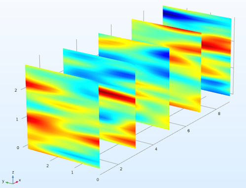
Input random field realization

Note the layered profile which is typical of most soil and rock and is obtained by specifying a relatively larger correlation length in horizontal plane (x and y directions) compared to the vertical (z) direction.  

The degree of saturation field obtained by transformation using the soil water retention variables for a given value of suction, and the corresponding electrical conductivity (obtained from Archie's law) distribution is shown below:

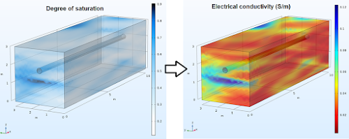
Transformed fields

An input realization can be used to generate a field for any soil or rock variable. I have shared below the Python code to generate random fields in 3D with the option to control properties such as field size, correlation lengths in 3 Cartesian coordinate axes, resolution of generated point cloud and rotation angle.  

The code may be directly pasted into a Jupyter notebook and the properties such as spatial correlation length in the three axes (x, y and z), the field size, resolution (points per meter) and the rotation angle can be changed according to requirements. When the code is run, a text file will be created at the specified location.

The code can be downloaded from : https://app.box.com/s/rfmypwlt88r0lysj8puj2bn8frqfkg2k

Another web app to estimate the soil water retention curve

I created another simple web application to estimate the soil water retention curve from basic particle size distribution data. I used the equations developed by Zapata et al. (2000). The water retention curve can be exported as before and the previous app can be used to estimate hydraulic conductivity and oxygen diffusion coefficient of the soil after fitting to the vanGenuchten model.

Link : https://rukshan-azoor-psd.anvil.app/

I have also embedded the app below:  

Building a web app with nothing but (a bit of) Python

My knowledge of Python (the programming language) is not extensive. I have used it a few times to streamline some of my research activities that include data handling and processing. I find Python easy to get into without much programming experience and sources like Stack Overflow help very much to do this. So when I came across a web platform called Anvil that claims to let you build fully functional web apps with nothing but Python, I decided to give it a try. I was pleasantly surprised, and happy with the web application that I was able to build with a relatively basic knowledge of Python and nothing else. My code may not be the most efficient, but it gets the job done.

I decided to build an app within my area of research. It is an app to estimate soil hydraulic properties and oxygen diffusion coefficients at different degrees of saturation, based on water retention properties of the soil. I used equations from literature and those developed in my own research to do this. Two water retention curve parameters (van Genuchten α and n) and the soil porosity are used as inputs and the hydraulic conductivity function and oxygen diffusion coefficient characteristic are generated using the equations. I used the Plotly library built into Anvil to generate three plots for the generated functions and the water retention curve. I also built in an option to export the generated data as a text file that can be used for further analysis.

I was able to do this with the free plan that Anvil offers. Anvil also has a paid subscription plan that has more Python libraries and more options for development support and deployment. I believe it is a great product with exciting capabilities.

My first web app can be accessed at :  https://rukshan-azoor-wrc.anvil.app/