For situations where 3D random fields are required, the user will have to generate their own fields and input into the software (if user inputs are allowed). For my work on corrosion in inhomogeneous soil, I generated 3D random fields and input the realizations into COMSOL Multiphysics as a point cloud. I used the excellent GeoStatTools (GSTools) Python library (Sebastian Müller & Lennart Schüler. GeoStat-Framework/GSTools. Zenodo.https://doi.org/10.5281/zenodo.1313628) for this purpose. This library can be used to generate random fields based on several covariance models. Once the random fields are generated using this method, the rest is simply data manipulation and formatting to match the input format for a particular software. For my purpose, I generated a random field based on the standard normal distribution (Mean=0, Std.dev=1) so that I can transform it to any soil property (including log-normally distributed parameters by transformation by log values). I formatted the output field as a text file containing columns for the three spatial coordinates and the corresponding density value from the random field. This file can be input as a point cloud to COMSOL.
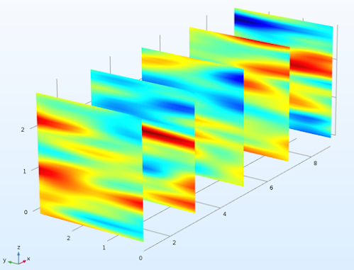
For example, the random field realization from a standard normal distribution after input to COMSOL is shown below:
 |
| Input random field realization |
Note the layered profile which is typical of most soil and rock and is obtained by specifying a relatively larger correlation length in horizontal plane (x and y directions) compared to the vertical (z) direction.
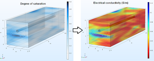
The degree of saturation field obtained by transformation using the soil water retention variables for a given value of suction, and the corresponding electrical conductivity (obtained from Archie's law) distribution is shown below:
 |
| Transformed fields |
An input realization can be used to generate a field for any soil or rock variable. I have shared below the Python code to generate random fields in 3D with the option to control properties such as field size, correlation lengths in 3 Cartesian coordinate axes, resolution of generated point cloud and rotation angle.
The code may be directly pasted into a Jupyter notebook and the properties such as spatial correlation length in the three axes (x, y and z), the field size, resolution (points per meter) and the rotation angle can be changed according to requirements. When the code is run, a text file will be created at the specified location.
The code can be downloaded from : https://app.box.com/s/rfmypwlt88r0lysj8puj2bn8frqfkg2k

Hello Rukshan. Thanks for sharing your script, it's helping me a lot. I've been searching about random fields and I saw that a lot of works in geotechnic used the Local Average Subdivision Method (LAS) to generate the fields. I looked that GSTools uses the randomisation method. By any chance, have you ever found any script of LAS in Python? Or studied the diferences between the methods? greetings, Natália
ReplyDeleteHello Natália,
DeleteYou're welcome. I haven't found a Python script that uses the LAS method to generate random fields, and am yet to study the different methods in detail. However, to my knowledge, the randomisation method is a modification of the Fast Fourier Transform (FFT) method.
This paper describes the randomisation method:
https://www.sciencedirect.com/science/article/pii/S1364815214000231
and this book outlines the various methods for random field generation, including LAS:
https://onlinelibrary.wiley.com/doi/book/10.1002/9780470284704
Hope this helps
Cheers
Rukshan
Dear Rukshan,
ReplyDeletefirst of al, thanks for the informative post. How did you produce those semi-transparent 3D volume plots?
Hello,
DeleteThanks. The 3-D volume plots were generated using the COMSOL Multiphysics software.
Thanks, Rukshan! One more question: you mention that you generate a standard normal distribution, form which (via transofrmations) you obtain the desired distribution for a specific property (e.g. saturation). Yet in your example code:
Deletemodel = Gaussian(dim=3, var=0.5, len_scale=[corrx*ppm, corry*ppm,corrz*ppm], angles=0.)
...you set the variance to 0.5. Just for my understanding - was this supposed to read var=1.0 or did I get something wrong?
Hello, Yes that is a mistake. It should read var=1.0. Thanks for pointing it out. I was playing around with the values and it seems I have saved the wrong version.
Delete