Spatial variability of soil and localised underground corrosion

Underground corrosion is a problem that often goes unnoticed, but has a significant economic impact. Corrosion of buried metallic infrastructure such as pipelines is highly variable, and can be influenced by many complex factors. In addition to phenomena such as stray currents and differential aeration that lead to rapid levels of corrosion, we have shown that the spatial variability, or heterogeneity of soil itself can lead to differential conditions that evolve into rapid localised corrosion.  

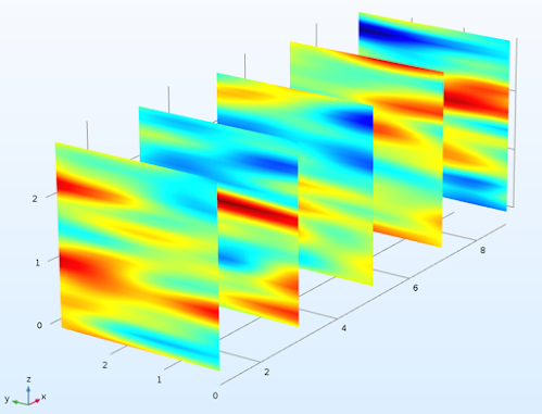
In a previous blog post I described how to create random field realisations using Python for various soil parameters with given statistical properties. The idea was to export these realisations as point clouds into numerical modelling software to simulate various processes under heterogenous soil conditions. When we simulated corrosion of buried metal in heterogenous soil using this method, we saw that the spatial variations in soil resulted in localised corrosion defects termed "corrosion patches" that evolve with time until failure occurs. In this context, failure is defined as the point when when the corrosion patch depth exceeds the pipe wall thickness. 

The emergence of localised corrosion from numerical modelling of spatially variable soil, similar to actual corrosion patches observed in the field 

However, running such simulations is computationally intensive, especially if multiple realisations over longer pipe lengths are needed to be simulated. To overcome this problem, we used Artificial Neural Networks (ANN). ANNs are a machine learning method that use a system of simulated neurons to identify and infer patterns from data without being given explicit instructions. It is similar to how neurons in our brains work, with a neuron having several inputs and is activated (similar to a neuron firing in the brain) when the weighted sum of the inputs exceed a certain threshold. An organised set of such neurons can "learn" to map input data to outputs by adjusting the weights and biases used for activation.   

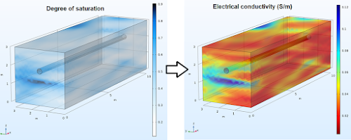
We identified two of the most influential soil properties that influence corrosion: degree of saturation and saturated electrical resistivity. We then trained an ANN using input data from random field realisations of these two variables and numerical model outputs of corrosion parameters for the same realisations. Through this method we developed an ANN that was capable of predicting the level of corrosion over time for given values of these input variables. We were now able to use this trained neural network to simulate corrosion over much longer pipe segments for multiple realisations with lower computational effort and time. We outlined this method and simulation results in a recently published paper: 

https://link.springer.com/article/10.1007%2Fs11440-021-01385-5

In this paper we show how the soil degree of saturation and resistivity influence the corrosion patch configurations. We also describe a linear approximation that can be adopted for assessing information along buried pipelines, and note that the workflow and methods used in this work can be adopted together with underground sensing methods for non-destructive pipeline condition assessment. 

Using Artificial Neural Networks together with numerical modelling to predict pipeline corrosion in spatially variable soil

Modelling soil inhomogeneity using 3D random fields - Python code

Soil properties are inherently variable and this variability needs to be factored in simulations and analysis. The spatial variability of soil can be modeled using realizations of random fields which can then be used for Monte Carlo simulations. While some software programs such as Rocscience Slide and Optum G2 offer random field analysis, they are restricted to 2D simulations and random field creation is often limited in flexibility.  

For situations where 3D random fields are required, the user will have to generate their own fields and input into the software (if user inputs are allowed). For my work on corrosion in inhomogeneous soil, I generated 3D random fields and input the realizations into COMSOL Multiphysics as a point cloud. I used the excellent GeoStatTools (GSTools) Python library (Sebastian Müller & Lennart Schüler. GeoStat-Framework/GSTools. Zenodo.https://doi.org/10.5281/zenodo.1313628) for this purpose. This library can be used to generate random fields based on several covariance models. Once the random fields are generated using this method, the rest is simply data manipulation and formatting to match the input format for a particular software. For my purpose, I generated a random field based on the standard normal distribution (Mean=0, Std.dev=1) so that I can transform it to any soil property (including log-normally distributed parameters by transformation by log values). I formatted the output field as a text file containing columns for the three spatial coordinates and the corresponding density value from the random field. This file can be input as a point cloud to COMSOL. 

For example, the random field realization from a standard normal distribution after input to COMSOL is shown below:

Input random field realization

Note the layered profile which is typical of most soil and rock and is obtained by specifying a relatively larger correlation length in horizontal plane (x and y directions) compared to the vertical (z) direction.  

The degree of saturation field obtained by transformation using the soil water retention variables for a given value of suction, and the corresponding electrical conductivity (obtained from Archie's law) distribution is shown below:

Transformed fields

An input realization can be used to generate a field for any soil or rock variable. I have shared below the Python code to generate random fields in 3D with the option to control properties such as field size, correlation lengths in 3 Cartesian coordinate axes, resolution of generated point cloud and rotation angle.  

The code may be directly pasted into a Jupyter notebook and the properties such as spatial correlation length in the three axes (x, y and z), the field size, resolution (points per meter) and the rotation angle can be changed according to requirements. When the code is run, a text file will be created at the specified location.

The code can be downloaded from : https://app.box.com/s/rfmypwlt88r0lysj8puj2bn8frqfkg2k