Modelling soil inhomogeneity using 3D random fields - Python code

Soil properties are inherently variable and this variability needs to be factored in simulations and analysis. The spatial variability of soil can be modeled using realizations of random fields which can then be used for Monte Carlo simulations. While some software programs such as Rocscience Slide and Optum G2 offer random field analysis, they are restricted to 2D simulations and random field creation is often limited in flexibility.  

For situations where 3D random fields are required, the user will have to generate their own fields and input into the software (if user inputs are allowed). For my work on corrosion in inhomogeneous soil, I generated 3D random fields and input the realizations into COMSOL Multiphysics as a point cloud. I used the excellent GeoStatTools (GSTools) Python library (Sebastian Müller & Lennart Schüler. GeoStat-Framework/GSTools. Zenodo.https://doi.org/10.5281/zenodo.1313628) for this purpose. This library can be used to generate random fields based on several covariance models. Once the random fields are generated using this method, the rest is simply data manipulation and formatting to match the input format for a particular software. For my purpose, I generated a random field based on the standard normal distribution (Mean=0, Std.dev=1) so that I can transform it to any soil property (including log-normally distributed parameters by transformation by log values). I formatted the output field as a text file containing columns for the three spatial coordinates and the corresponding density value from the random field. This file can be input as a point cloud to COMSOL. 

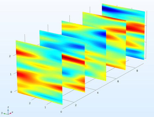
For example, the random field realization from a standard normal distribution after input to COMSOL is shown below:

Input random field realization

Note the layered profile which is typical of most soil and rock and is obtained by specifying a relatively larger correlation length in horizontal plane (x and y directions) compared to the vertical (z) direction.  

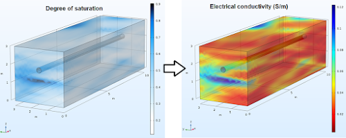
The degree of saturation field obtained by transformation using the soil water retention variables for a given value of suction, and the corresponding electrical conductivity (obtained from Archie's law) distribution is shown below:

Transformed fields

An input realization can be used to generate a field for any soil or rock variable. I have shared below the Python code to generate random fields in 3D with the option to control properties such as field size, correlation lengths in 3 Cartesian coordinate axes, resolution of generated point cloud and rotation angle.  

The code may be directly pasted into a Jupyter notebook and the properties such as spatial correlation length in the three axes (x, y and z), the field size, resolution (points per meter) and the rotation angle can be changed according to requirements. When the code is run, a text file will be created at the specified location.

The code can be downloaded from : https://app.box.com/s/rfmypwlt88r0lysj8puj2bn8frqfkg2k

Another web app to estimate the soil water retention curve

I created another simple web application to estimate the soil water retention curve from basic particle size distribution data. I used the equations developed by Zapata et al. (2000). The water retention curve can be exported as before and the previous app can be used to estimate hydraulic conductivity and oxygen diffusion coefficient of the soil after fitting to the vanGenuchten model.

Link : https://rukshan-azoor-psd.anvil.app/

I have also embedded the app below:  

Building a web app with nothing but (a bit of) Python

My knowledge of Python (the programming language) is not extensive. I have used it a few times to streamline some of my research activities that include data handling and processing. I find Python easy to get into without much programming experience and sources like Stack Overflow help very much to do this. So when I came across a web platform called Anvil that claims to let you build fully functional web apps with nothing but Python, I decided to give it a try. I was pleasantly surprised, and happy with the web application that I was able to build with a relatively basic knowledge of Python and nothing else. My code may not be the most efficient, but it gets the job done.

I decided to build an app within my area of research. It is an app to estimate soil hydraulic properties and oxygen diffusion coefficients at different degrees of saturation, based on water retention properties of the soil. I used equations from literature and those developed in my own research to do this. Two water retention curve parameters (van Genuchten α and n) and the soil porosity are used as inputs and the hydraulic conductivity function and oxygen diffusion coefficient characteristic are generated using the equations. I used the Plotly library built into Anvil to generate three plots for the generated functions and the water retention curve. I also built in an option to export the generated data as a text file that can be used for further analysis.

I was able to do this with the free plan that Anvil offers. Anvil also has a paid subscription plan that has more Python libraries and more options for development support and deployment. I believe it is a great product with exciting capabilities.

My first web app can be accessed at :  https://rukshan-azoor-wrc.anvil.app/